Appropriate models for 3D motion analysis
May 16, 2017
Embedded motion engineers have to know how the smart electronics get placed within the physical structure (“embedded”) and how each component moves relative to each other (“motion”). In this...
Embedded motion engineers have to know how the smart electronics get placed within the physical structure (“embedded”) and how each component moves relative to each other (“motion”). In this article, I’d like to discuss how we describe and model the latter term, motion, which we often take for granted as being quite simple.
When we design motion systems, we ask things like:
- Is the motion stable?
- How can we make the motion smoother and more elegant?
- What’s the best way to achieve the desired motion?
To answer these questions with high technical predictability, we often enlist trusted kinematic and dynamic models. Sometimes the models we find in the Machinery’s Handbook, the Engineering ToolBox, Wikipedia, or elsewhere on the engineering web will be sufficient models for our scenario. Sometimes, they don’t hold water, and we need a model with stronger predictive capabilities.
An oft-quoted engineering saying goes, “All models are wrong. Some are useful.” No doubt, the tenet also applies to 3D motion. Some kinematic and dynamic models can be appropriate in one scenario, but insufficient in other scenarios.
For motion, the universally applicable equations can handle multidirectional 3D rotating and translating bodies, while the simple equations can only handle translation and unidirectional rotation. The simple equations can be appealing because they’re quick and easy. I’ll illustrate this idea below by comparing two systems that require different approaches for appropriate kinematic models.
Simple motion analysis
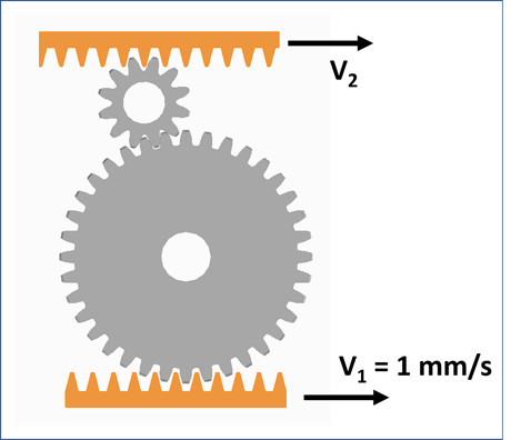
The diagram below shows a simple gear system. The bottom rack is driving the two gears and another rack. Let’s assume the centers of the two gears are fixed, so that the gears are only rotating, and the top rack is moving in the x-direction. If the bottom rack is moving at ν1 = 1mm/s, how fast is the top rack moving (assuming no loss in the gears)?
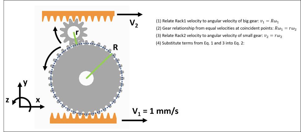
It turns out the equations we need are quite straightforward. We can easily define angular information in this example:
- The angular velocity (ω) of each gear is equal to the time rate of change of just one angle (θ). For the larger gear, for example, we can say that its angular velocity is described by ω1 = θ̇1.
- Each of the gears is rotating about its center of mass.
By essentially treating this system as 2D, we’re safe to use ν = τω in our analysis. Applying the relationship to design our system yields that ν2 = ν1.
Moving to 3D
What do we do when we encounter 3D motion systems that have parts rotating in more than one direction and not about their center of mass? How do we define the angles? What is the angular velocity?
The motion of a quadcopter is a suitable example of a more complicated 3D motion system. For a quadcopter, we want stable control over its position (“Where is it located? How fast is it going?”) and orientation in space (“What’s the ‘tilt’ angle?”). It’s possible for a quadcopter in flight to translate in x, y, and z directions and rotate about x, y, and z (where x-y-z are three orthogonal directions fixed in the space).
To keep the quadcopter stable, we’ll use a gyroscope to measure the angular velocity about each axis, and feed that information back into the control algorithm. A 3-axis gyroscope will spit out three values for angular velocity, but note that these angular velocities correspond to axes that are fixed on the quadcopter. These x-y-z axes are not the same as the x-y-z axes that relate back to the quadcopter’s position, velocity, and acceleration in space. The conversion, so to speak, of the gyroscope’s output into something digestible by the control algorithm is where the 3D dynamics model comes in handy.
Getting started with a more powerful 3D model
A more robust model of 3D motion starts with:
- Assigning a reference frame to a point fixed in your space.
- Treating all the objects in your system as rigid bodies.
- Assigning a reference frame to a certain point on each body.
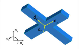
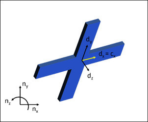
A reference frame is what I’m calling a set of three orthogonal unit vectors attached to a certain point. For this example, the only object is the quadcopter, so we’ll treat that as a single rigid body. (We’ll ignore the other parts on the quadcopter here.) We’ll say that a reference frame N is fixed at a point on the earth and is made up of n̂x, n̂y, and n̂z. We’ll attach a reference frame D to the center of mass of the quadcopter. Reference frame D is made up of d̂x, d̂y, and d̂z. The diagram above shows a simplified depiction in CAD.
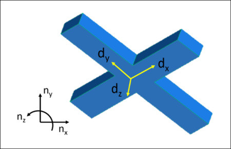
The measurements from the gyroscopes will give us angular velocities about d̂x, d̂y, and d̂z, and for the control algorithm, we’ll want to know how these values relate to meaningful angles in n̂x, n̂y, and n̂z. One way to achieve this is by defining the quadcopter’s orientation with a series of simple rotations about axes fixed on the quadcopter body. At the beginning of this step, we can express the angular velocity of the quadcopter in d̂x, d̂y, and d̂z, and it will look something like this:
![]()
At the end of this work, we’ll use rotation matrices to express each of the angular velocities in terms of Euler angles. Euler angles provide us one way of precisely describing the orientation of a body in 3D space. (Note that Euler angles don’t necessarily correspond to what we call yaw, pitch, and roll.) We will finish with precise expressions for ω1, ω2, and ω3.
Since the quadcopter can rotate about more than one axis, we no longer have a simple ω1 = θ̇ relationship, and we can’t use ν = τω to generally describe the velocity of a point on a quadcopter. In fact, an equation for ω1 looks like ω1 = φ̇ = cos α + α̇ - θ̇ sin φ where θ, φ, and α are the Euler angles. The equations for ω2 and ω3 are no less messy, unfortunately. In short, it’s easy to see how the definition of the 3D system extends beyond what we find in traditional dynamics resources. For more details on these calculations, see the extra credit section.
Modeling complex motion phenomena
When we model complicated 3D motion phenomena, it’s key to distinguish between scalar and vector quantities. Remember, a vector has both a magnitude and direction (e.g., 25 mph in the northeast direction), while a scalar is something that just has a magnitude (25 mph). When we bring into our model other physical values (velocities, accelerations, linear and angular momentum, forces, torques, and so forth), we should first think of them as vector quantities. For instance, when we talk about torque, it’s useful to specify both its direction (e.g., about the positive z-axis), as well as its magnitude (5 N-m).
The benefit of using a more complex model is that you can precisely define all the quantities related to angles (the orientation, angular momentum, moments, and products of inertia, and so forth) for any motion system made up of rigid bodies. The equations can get gnarly, so it’s often wise to use software programs like MATLAB, Working Model, or MotionGenesis.
Note that if I were following the 3D model methodology in my gear example, then I would explicitly treat the velocity and angular velocity as vector quantities. But again, the motion in the gear example fits my criteria for simplifying down to 2D kinematic equations, and I avoid the time-heavy definitions of a 3D model. If I have a more complex motion system, then I must treat the kinematic and dynamic quantities as vectors, or I risk having a poorly predictive model.
Precisely modeling the motion of a system can be a tricky thing, but by constructing a robust model we can more quickly respond to broader concerns. If we desire to make a stable motion system that is functionally robust, smooth, and elegant, then we have to decide which model is more appropriate. As engineers, it’s critical for us to realize the limitations of the commonplace 2D equations, and that there are other appropriate tools to solve 3D motion systems.
For more resources and support for topics related to 3D motion analysis, follow Simplexity’s product development blog.
Extra Credit
Here is one way to precisely define rotational information for the quadcopter:
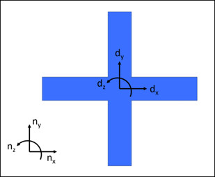
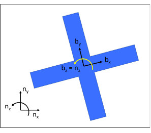
We’ll use intermediate reference frames to describe the orientation of the quadcopter. We’ll call the initial reference frame attached to the quadcopter B. Initially, b̂x= n̂x, b̂y= n̂y, and b̂z= n̂z. Reference frame D is still attached to the body, and initially, d̂z = b̂z= n̂z. We will rotate first about b̂z (which here is equal to d̂z), and we will rotate by angle +θ. We can then write that B’s angular velocity in N is ![]() .
.
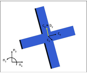
We will then rotate about another fixed axis on the body, d̂y, and we’ll call this new intermediate reference frame C. Initially, ĉx = b̂x, d̂y = ĉy = b̂y, and ĉz = b̂z. We’ll rotate by angle +φ about ĉy. We can then write that C’s angular velocity in B is ![]() .
.
Last, we will rotate about the fixed axis d̂x. Initially, d̂x = ĉx, d̂y = ĉy, and d̂z = ĉz.We’ll rotate by angle +α about d̂x. We can then write that D’s angular velocity in C is ![]() .
.
From here, D’s angular velocity in N can be expressed as ![]() . However, this expression isn’t very useful yet in putting together dynamic equations. We already know that
. However, this expression isn’t very useful yet in putting together dynamic equations. We already know that ![]() because that’s the format of the data coming from the gyroscope. We’d like to re-express this in terms of our global reference frame N.
because that’s the format of the data coming from the gyroscope. We’d like to re-express this in terms of our global reference frame N.
Thankfully, each of those rotations created a rotation matrix between each of the intermediate frames, and we can use the multiplication of those rotation matrices to express ![]() in terms of our defined angles. (I won’t go into details with this part, but it comes straight out of making those intermediate rotations.) The result is the following:
in terms of our defined angles. (I won’t go into details with this part, but it comes straight out of making those intermediate rotations.) The result is the following:
![]()
Note that we can arrive at an expression for ⍵1, ⍵2, and ⍵3 and in terms of θ, φ, and α and their derivatives (as shown in the main part of the text) by expressing this equation in terms of in d̂1, d̂2, and d̂3. Additionally (by doing some more rearranging), we can express each of the Euler angles in terms of ⍵1, ⍵2, and ⍵3. For example:
![]()
Alas, our first step in giving a precise definition for the angular velocity of the quadcopter and making it usable by the control algorithm is complete.