Profiling Java Applications on Embedded Platforms
August 26, 2019
Blog

My article is devoted to the consideration of a solution tested through practice that solves all the problems having to do with tools for profiling Java applications.
The rapid development of the gadgets market, both user and industrial, demands higher standards in gadget performance optimization. From wearable medical devices and car on-board computers to server racks and production lines, all devices must undergo performance optimization while taking into account the characteristics of electronics and executable software. Performance issues are most acute for Java applications. The problem of profiling on embedded platforms without significantly affecting application operation and not stopping its work is significant. Sometimes, it is necessary to conduct profiling in a production environment.
There are many tools for profiling Java applications. However, while some popular software simply does not provide this feature, most tools have several limitations, for example:
- When profiling a Java application, the tool might introduce distortions into the program because some part of the processing time is taken by the profiler itself. For example, in my work I had to deal with several cases of application operation damage. As a result, the developer did not see a real picture of application operation, but a very approximate one. It is often impossible to make the right decision based on such data.
- Java profilers cannot show the behavior of the Java Virtual Machine (JVM) itself, the garbage collector (GC), and the JIT compiler.
- Sometimes it is necessary to perform profiling on embedded platforms in a production environment without significantly affecting the operation of the application and without stopping the work. Many popular tools simply do not provide such ease in operability.
My article is devoted to the consideration of a solution tested through practice that solves all the problems mentioned above. For profiling Java applications on embedded platforms without performance loss and without distorting the received data, the most successful method will be to use multiple tools, namely: Linux perf, perf-map-agent, and FlameGraphs.
- Perf does not have the drawbacks described above, but it cannot determine JITed Java code; perf-map-agent comes to its aid in this situation.
- Perf-map-agent is a Java agent that connects to a virtual machine and generates JIT code mapping files for perf.
- Subsequently, the data collected by perf is processed using FlameGraphs and is displayed as diagrams, which are convenient for analyzing various data, for example, instructions executed, CPU cycles spent, cache hits, cache misses, and branch misprediction. The range of displayed parameters depends on what features the CPU offers for perf.
Below is an example of such a diagram with a stack of calls, where each call is aligned with a rectangle and its width is the number of collected samples (Fig. 1).
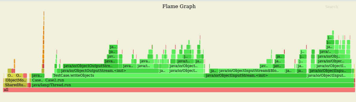
(Source: Auriga Inc.)
The implementation of this decision stack is described in further detail.
Step # 1: installing perf on Linux (Ubuntu, Debian).
$ apt-get install linux-perf
Step #2: configuring the kernel to access perf counters.
Allow all users to use perf
$ echo 0 | sudo tee /proc/sys/kernel/perf_event_paranoid
Let users get kernel characters
$ echo 0 | sudo tee /proc/sys/kernel/kptr_restrict
The general methodology for using perf is as follows.
Step #3: getting a list of supported event counters.
$ perf list
Step #4: querying high level statistics.
The statistics are saved for the specified process identifier PID to a file.
$ perf stat -d -d -d -p $PID sleep 10 > perf_stat_ddd.txt 2>&1
This data will show the high-level statistics of the application, which the developer can use to understand where the problem lies, such as in the CPU front-end, the CPU back-end, or even that the processor is not a bottleneck. Bottleneck can happen when an application is limited by network capacity or disk speed.
For example:
Performance counter stats for process id '1018':
80?007,47 msec cpu-clock # 8,000 CPUs utilized
23?065 context-switches # 288,287 M/sec
500 cpu-migrations # 6,249 M/sec
363?086 page-faults # 4538,178 M/sec
34?737?200?848 cycles # 434177,020 GHz (30,73%)
81?315?387?195 instructions # 2,34 insn per cycle (38,45%)
14?868?912?156 branches # 185845140,500 M/sec (38,48%)
136?313?613 branch-misses # 0,92% of all branches (38,53%)
17?790?132?862 L1-dcache-loads # 222357204,520 M/sec (38,56%)
326?141?420 L1-dcache-load-misses # 1,83% of all L1-dcache hits (38,56%)
64?401?058 LLC-loads # 804942,793 M/sec (30,80%)
19?811?845 LLC-load-misses # 30,76% of all LL-cache hits (30,76%)
251?303?204 L1-icache-load-misses (30,72%)
17?438?022?455 dTLB-loads # 217956209,519 M/sec (30,72%)
6?546?801 dTLB-load-misses # 0,04% of all dTLB cache hits (30,72%)
4?009?666 iTLB-loads # 50116,440 M/sec (30,72%)
2?507?515 iTLB-load-misses # 62,54% of all iTLB cache hits (30,72%)
10,001317995 seconds time elapsed
By looking at the table more closely, we can decipher what the data indicate. Firstly, it is worth paying attention to the two key values: “cycles” and “instructions.” These counters show how many cycles and instructions were executed by the processor for a certain time interval. One of the key metrics in analyzing application performance is the ratio of executed instructions to cycles, and namely:

The higher the IPC value, the better. On modern processors, IPC can be higher than 1, that is, more than one instruction can be executed in a single clock cycle.
With the above example, IPC = 2.34, which is already a pretty good result. Using the IPC, which way to go can be determined.
For the current example:
First, ensuring that the application takes up 100 percent of the processor time and at the same time, does useful work that is necessary. Currently, only 8 percent of the CPU is used.
Secondly, attention must be paid to LLC-load-misses: in the current example, misses in the Last Level Cache account for 30 percent of hits. In the future, this metric should be taken for a more detailed study and a flame graph should be built for it. Below are details on how to do this.
In general, the developer needs to remember that the processor pipeline has a front-end and a back-end. The front-end performs the first part of the work—fetching instructions, predicting branching, and decoding instructions in microoperation (uOps). Thus, metrics such as branch-misses, L1-icache-load-misses show front-end problems.
The back-end sends micro-operations to execution units for execution. At this stage, everything must be ready for a microoperation to be executed: the cache must contain the necessary data, and the executive units must be free. In this case, the metrics L1-dcache-load-misses, LLC-load-misses will show problems in the back-end.
Perf has two counters specifically for problems on the back-end and the front-end:
stalled-cycles-frontend
stalled-cycles-backend
Step #5: getting an application profile with hot methods.
Recording functions belong to the PID process that take up processor time, with a frequency of 99 Hz, for 10 seconds:
$ perf record -F 99 -p $PID sleep 10
To record a stack of functions occupying the processor, for example, recording with frequency of 99 Hz, for 10 seconds:
$ perf record -F 99 -ag -- sleep 10
As a result of execution, a perf.data file will appear.
Step #6: indication of a specific event.
How to record statistics for misses in the CPU cache—record every hundredth miss from the whole system for 10 seconds:
$ perf record -e cache-misses -c 100 -a -- sleep 10
Step #7: viewing results in the console interface.
Having received the perf.data file, open it in the console with the $ perf report command.
List of symbol values ??in the received report:
[.] : user level
[k]: kernel level
[g]: guest kernel level (virtualization)
[u]: guest os user space
[H]: hypervisor
Step #8: JVM profiling.
To profile Java applications, you need an agent, which I suggest downloading from github:
The build is gathered as follows:
$ cmake .
$ make
There are at once several helper scripts in bin for running perf, for example, to gather perf.data:
$ ./bin/perf-java-report-stack.sh $PID $PERF_OPTIONS
There is also a script to generate a call chart:
$ ./bin/perf-java-flames.sh $PID $PERF_OPTIONS
Step #9: manual creation of FlameGraph diagrams.
The first step is to get the latest FlameGraph:
Then, having a perf.data file, combine the stacks of the same methods:
$ perf script | ../FlameGraph/stackcollapse-perf.pl > perf.collapsed
Now an application profile can be made:
$ ../FlameGraph/flamegraph.pl perf.collapsed > profile.svg
To get a more accurate picture of the profile, the option to save the stack frame sometimes helps. To do this, adding the –XX: + PreserveFramePointer option to the Java application is required and start profile recording, for example:
$ java -XX:+PreserveFramePointer -jar myapp.jar &
$ ./perf-map-agent/bin/perf-java-report-stack.sh $JAVA_PID $PERF_OPTIONS
To summarize the step, the bundle of perf + perf-map-agent + FlameGraphs tools allows you to study the work of not only the application itself, but also the JVM. Data can be obtained to improve the performance of the GC or other components of the JVM. These tools help, even if the performance problem lies in the operating system itself.