
Are Random Numbers in LTspice Truly Random?
September 04, 2025
Blog
This article discusses how to include pseudorandomness and true randomness in LTspice® simulations using the flat(), gauss(), and mc() functions, as well as how to use the Use the clock to reseed the MC generator option in the Hacks section of the settings panel. Trade-offs between pseudorandomness and true randomness are discussed, as well as trade-offs between statistical, Monte Carlo-like simulations and more targeted worst-case simulations.
Introduction
There are a few options to simulate randomness in an LTspice® schematic. The flat(), gauss(), and mc() functions in LTspice enable randomness in LTspice simulations. The mc() function is used throughout this article to illustrate how to simulate passive component value tolerances. With LTspice open, select Help > LTspice Help (or press F1) to open the Help Manual for more information on flat() and gauss().
In the example in Figure 1, mc() is used to set the nominal value and tolerance of R1 and C1. For example, the nominal value for R1 is 10 kΩ, and the tolerance is 5%. The mc(x,y) function will generate pseudorandom numbers with uniform distribution between x*(1-y) and x*(1+y). Keep reading to learn more about the distinction between pseudorandom and truly random numbers, and how to force LTspice to generate truly random numbers. The .STEP directive is used to instruct LTspice how many iterations of the simulation to run. In the following example, the .STEP directive steps a dummy parameter from 1 to 100 in increments of 1, resulting in 100 simulation runs where the values of R1 and C1 are both randomized.
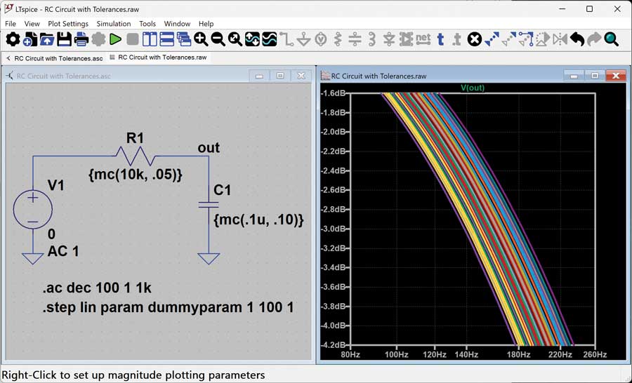
Figure 1. RC circuit using mc() to set value and tolerances of passive components.
Observe what this mc() function is doing during each step iteration: Figure 2 shows a simpler example using a voltage source only. This example uses mc() to set the nominal voltage to 10 V and the tolerance at 100%, so a uniform distribution between 0 V and 20 V is expected. From the results in the waveform viewer and in the SPICE output log, notice that for 10 iterations, the voltage varies from 2.7 V to 19.92 V, and the distribution isn’t entirely uniform, but more iterations would help to ensure that these results are more statistically sound.
Taking an even closer look, try running this simulation several times. Do you see the numbers change at all during these simulations? On my computer, every time I run this, I get the same voltages for each step iteration. Not very random, is it?
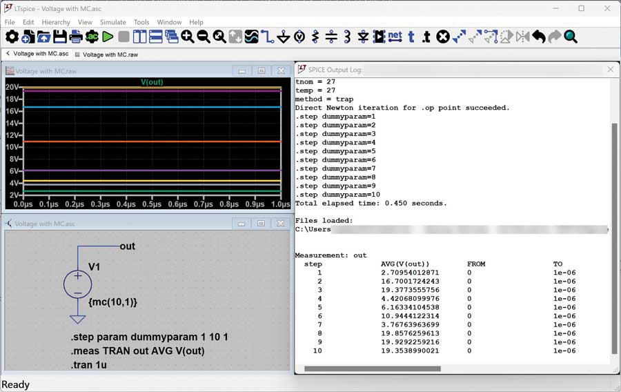
Figure 2. Voltage source using mc() to randomize voltage.
What you’re observing is classic behavior in code and computers when generating random numbers. Random number generators in programming languages have an optional seed() method associated with them. For a truly random number—one that changes each time you run the program—you’ll want to call the seed() method with a seed value that varies from run to run. Oftentimes, the programmer will pass the current system time to the seed() method to achieve this randomness.
How does this relate to our LTspice simulation? If the goal is true run-to-run randomness in the simulation—meaning, values that change during each simulation—the Use the clock to reseed the MC generator option must be enabled in the Hacks section of the settings panel (see Figure 3).
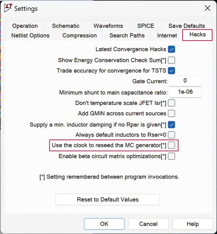
Figure 3. Hacks tab of LTspice Settings panel, showing how to turn on run-to-run randomization.
This uses the clock to reseed the MC generator option works for the flat() and gauss() functions as well. These functions can be used in the same places that mc() is used.
That said, think twice about whether this is simulation behavior that you want to implement intentionally. Do you want your simulation to be truly random? If so, you will lose predictability and repeatability in your simulation.
To illustrate, let’s look back at the example in Figure 2. What if the intention is to simulate a voltage that has a uniform distribution between 0 V and 20 V? The current example doesn’t quite meet expectations; however, getting much closer is possible by increasing the number of iterations from 10 to 100 (Figure 4). This adjustment brings the simulation much closer to achieving the desired distribution edges.
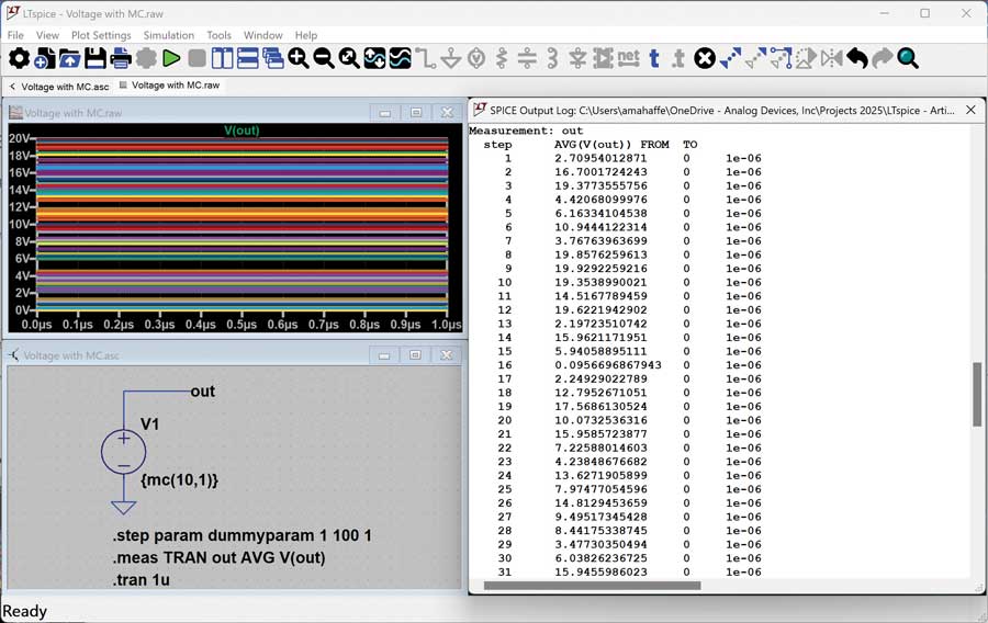
Figure 4. Voltage source using mc() with a higher number of iterations.
Now it is clear that (a) 100 iterations of mc() is going to result in a pretty good distribution of values, and (b) without enabling the reseed the MC generator hack, that result is going to be repeatable every time the simulation runs.
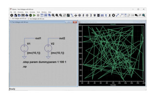
What if mc() is used in multiple places in the circuit? Can it be guaranteed that all the tolerance corners are hit with 100 iterations? Figure 5 illustrates this attempt, showing two voltage sources using mc(). Plotting V(out1) and setting the x-axis to V(out2), it’s clear that the combinations of V1 and V2 hit a fairly random set of coordinates (right-click on the x-axis title to change the x-axis from the stepped dummy parameter to V(out2)). But, technically, the minimums and maximums of these voltages are not being hit simultaneously, leading to some lack of coverage at the corners.
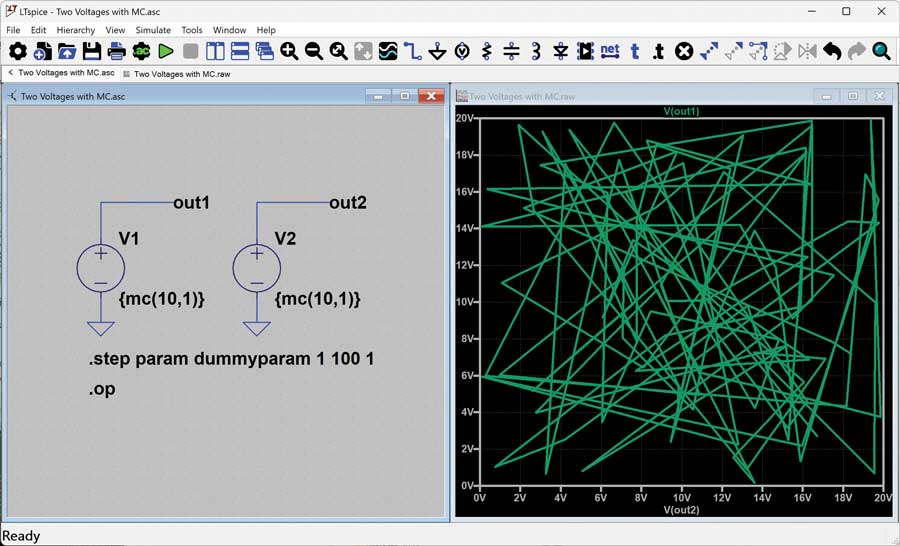
Figure 5. Plotting the results of two mc() voltages in one simulation.
More step iterations are needed if the goal is to get closer to complete coverage (Figure 6).
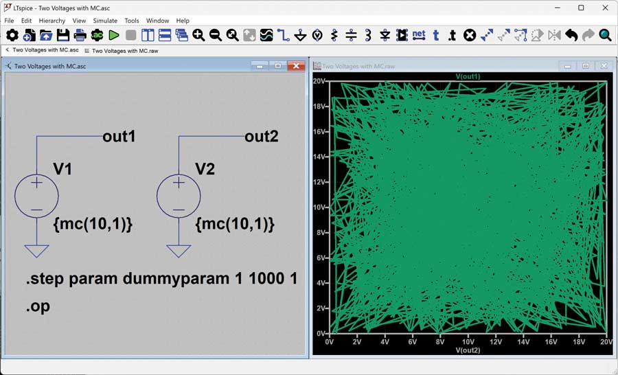
Figure 6. Plotting the results with more iterations.
For this simple example, the simulation runs quickly, so there is no concern with running this simulation 1000 times. What if a simulation takes a long time to run, and it would take hours (or days) to run a simulation with that many iterations? And consider the possible value of turning on the Use the clock to reseed the MC generator. If it is determined that the values generated by mc() in a simulation run are satisfactory, is the goal to have those results repeatable from run to run? Or is the preference for them to change randomly between simulation runs? It’s a great question to consider before enabling this hack setting.
In the interest of dramatically reducing simulation time, let’s explore a less random approach.
Figure 7 shows an example ensuring that the simulation hits all edges of the passive component tolerances while keeping the overall simulation time minimal. This example steps through three values of R1 and three values of C1, resulting in nine simulations, and it ensures that scenarios are covered for simultaneous minimums (or maximums) in the component values.
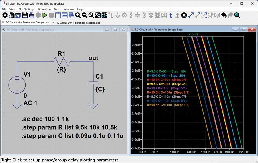
Figure 7. Setting specific values for components to simulate behavior due to tolerances.
Conclusion
If the goal is to explore a circuit across the corners of operation, a less randomized approach might make the most sense. If, instead, the aim is to perform a statistical analysis of how the simulation will behave across a range of variations, using a large number of simulations combined with functions that introduce randomness might be the best approach. Either way, you now have a better understanding of how to include some randomness (or not) in your LTspice simulation.
For more information, read the article “How to Model Statistical Tolerance Analysis for Complex Circuits Using LTspice.”
Anne Mahaffey joined Analog Devices in 2003 as a test engineer supporting direct digital synthesis products after receiving her B.S.E.E. from the Georgia Institute of Technology and her M.S.E.E. from North Carolina State University. She spent over 10 years architecting and supporting design tools in the Precision Studio tool suite and now supports LTspice® as a principal applications engineer.

Anne Mahaffey joined Analog Devices in 2003 as a test engineer supporting direct digital synthesis products after receiving her B.S.E.E. from the Georgia Institute of Technology and her M.S.E.E. from North Carolina State University. She spent over 10 years architecting and supporting design tools in the Precision Studio tool suite and now supports LTspice® as a principal applications engineer.